NeurIPS-2020 Deep Graph Contrastive Representation Learning
GRACE: Node-Level Unsupervised Graph Contrastive Learning
Abstract
The authors propose a node-level unsupervised contrastive representation learning framework. Two views are produced via corruption, and node representations are learned by maximizing agreement between node embeddings across the two views.
They introduce a mixed scheme for generating graph views at both the structural and attribute levels.
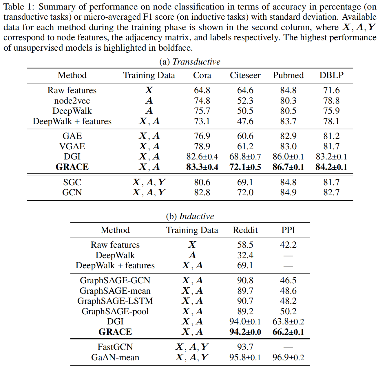
Experiments show that, despite its simplicity, the method substantially outperforms current state-of-the-art approaches on both transductive and inductive learning tasks.
Introduction
This work is motivated by DGI (Deep Graph InfoMax), which defines an objective based on maximizing mutual information (MI) on graphs.
- A GNN is first used to learn node embeddings, followed by a global summary embedding (graph embedding).
- The goal is to distinguish nodes in the original graph from nodes in a corrupted graph, thereby maximizing MI between node embeddings and the graph embedding.
- Limitations:
- DGI employs a mean-pooling readout function, which does not ensure that the graph embedding can extract useful information from nodes, because it is insufficient to preserve distinctive characteristics from node-level embeddings.
- DGI uses feature transformations to construct corrupted views. When generating negative node samples, however, this scheme corrupts node features at a coarse granularity. When the feature matrix is sparse, feature transformation alone is inadequate to produce distinct neighborhoods (i.e., contexts) for nodes in the corrupted graph, which makes learning the contrastive objective difficult.
This paper presents a simple yet effective framework for unsupervised graph contrastive learning. Rather than contrasting nodes against a global summary, it focuses on node-level contrast.
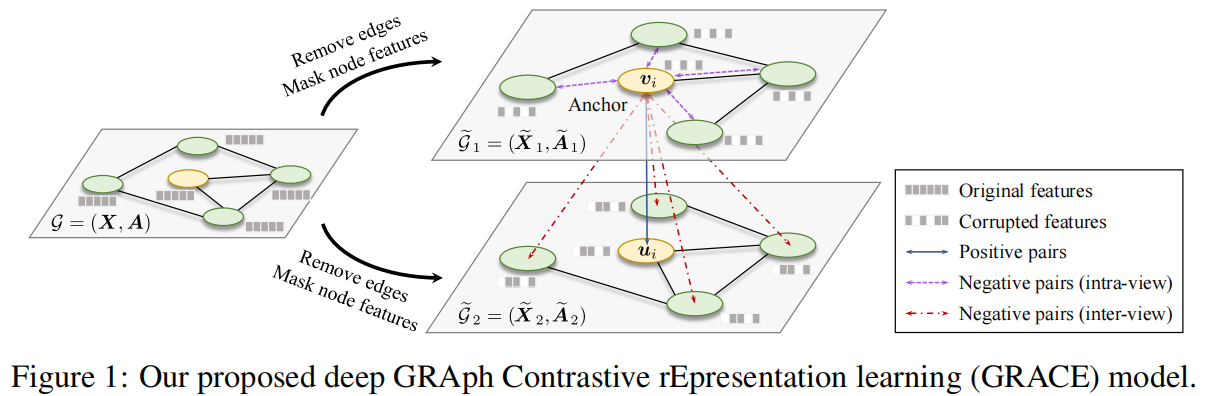
- Two correlated graph views are generated through random corruption operations, and consistency between views is maximized.
- Corruption is applied at both the topology and node-attribute levels, namely edge removal and feature masking.
Model
Preliminaries
$\mathcal{G}=(\mathcal{V},\mathcal{E}),\mathcal{V}=\{v_1,v_2,\cdots,v_N\},\mathcal{E}\subseteq\mathcal{V}\times\mathcal{V}$
Feature matrix: $X\in \mathbb{R}^{N\times F}$, where $x_i\in \mathbb{R}^F$.
Adjacency matrix: $A\in \{0,1\}^{N\times N}$; $A_{ij}=1$ when $(v_i,v_j)\in \mathcal{E}$.
No node class labels for $\mathcal{G}$ are available during training. The objective is to learn a GNN encoder $f(X, A)\in \mathbb{R}^{N\times F'}$ that takes graph structure and features as input and outputs low-dimensional node representations.
Let $H=f(X,A)$ denote the learned representations, with $h_i$ the embedding of node $v_i$.
Contrastive Learning of Node Representations
Each iteration constructs two views, $G_1$ and $G_2$, and computes view-specific node embeddings $U=f(X_*,A_*)$.
The same node in the two views forms a positive pair; all other nodes serve as negatives. With $M$ nodes, there are $2M-2$ negative samples.
Graph View Generation
Two operations:
- RE (Removing edges)
- Randomly delete a subset of edges.
- Sample a random mask matrix: if
$A_{ij}=1$in the original graph, its entry is drawn from a Bernoulli distribution$R_{ij}\sim \mathcal{B}(1-p_r)$; otherwise$R_{ij}=0$. The resulting adjacency matrix is$\tilde{A}=A\circ R$.
- MF (Masking node features)
- Randomly zero out feature dimensions at each node.
- Sample a random vector
$m\in \{0,1\}^F$, with each dimension drawn independently from a Bernoulli distribution with success probability$1-p_m$. Corrupted node features are$\tilde{X}=[x_1\circ m;x_2\circ m;\cdots,x_N\circ m]^T$.
The RE and MF schemes are technically analogous to DropEdge and feature dropout. Experiments indicate that the model is relatively insensitive to the choice of $p_r$ and $p_m$ under mild settings, so the original graph is not excessively corrupted.
Experiment