ICML-2020 Contrastive Multi-View Representation Learning on Graphs

2020-06-13 · ICML· ML · contrastive-learning, GNN

Paper: Contrastive Multi-View Representation Learning on Graphs

Contrastive learning on different structural views of graphs for graph classification

Abstract

Representations at the node and graph levels are learned by contrasting structural views of graphs. Unlike visual representation learning, increasing the number of views beyond two or contrasting multi-scale encodings does not improve performance; contrasting encodings of first-order neighbors and graph diffusion yields the best results.

The authors achieve state-of-the-art on all 8/8 node and graph classification benchmarks, outperforming supervised baselines on 4/8.

Introduction

Well-designed graph neural networks can handle graphs of variable size with permutation invariance. They learn low-dimensional embeddings by iteratively passing, transforming, and aggregating information; each iteration expands the receptive field by one hop, so after (k) iterations a node aggregates influence from nodes within (k) hops.

GNNs often rely on task-specific labels to learn deep (rich) representations, but annotating graphs is difficult: graphs are domain-specific, unlike common modalities such as video, images, or text, and labeling requires domain expertise and is costly. To address this, self-supervised methods—such as reconstruction-based or contrastive approaches combined with GNNs—can learn without labeled data.

Recent work achieves state of the art on node and graph classification by contrastive learning that maximizes mutual information between node and graph representations, but these methods depend on specialized encoders.

Recent progress in multi-view visual representation learning relies on data augmentation: obtaining multiple views of an image for contrastive learning has reached state of the art and surpassed supervised learning on image classification, but it is not yet clear whether this paradigm transfers to graphs.

This paper trains graph encoders by maximizing mutual information between representations encoded from different structural views of the same graph. The authors argue that the approach does not require a task-specific architecture and substantially outperforms prior models.

They systematically study the main components of this framework and find differences from visual contrastive learning:

Increasing the number of views beyond two does not help; the best setup contrasts first-order neighbors and graph diffusion.
Cross-view contrast between node and graph encodings works better than graph–graph or multi-scale encodings.
A simple readout layer outperforms complex architectures such as DiffPool.
Aside from early stopping, other regularization and normalization hurt performance.

With these design choices, they achieve state-of-the-art results.

Unsupervised Representation Learning on Graphs

Random walk: flatten nodes into sequences via random walks.

Graph kernels: decompose graphs into subgraphs and measure similarity with kernel functions.

Graph autoencoders (GAE): train an encoder to map graphs to latent vectors and predict first-order neighbors.

Graph Diffusion Networks

Graph diffusion networks (GDN) combine spatial message passing with generalized graph diffusion, where diffusion acts as a denoising filter that allows information to flow through higher-order neighbors. Early-fusion and late-fusion variants exist.

Learning by Mutual Information Maximization

InfoMax trains encoders to learn representations by maximizing mutual information, but the choice of encoder and mutual information estimator also strongly affects performance.

Method

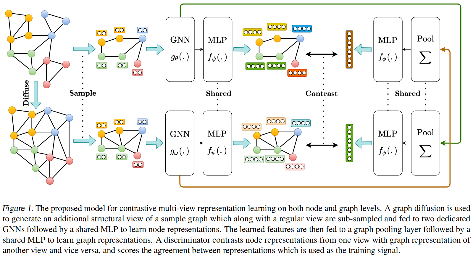
Main components:

Data augmentation: transform a sampled graph into two correlated views, augmenting structure only (not initial node features). A sampler then subsamples the same nodes from both views, analogous to cropping in computer vision.
Two view-specific graph encoders, each followed by a shared MLP projection head to learn node representations for the two views.
Graph pooling (readout), followed by a shared MLP projection head to learn graph-level representations for both views.
Discriminator: scores agreement by contrasting node representations from one view with graph representations from the other.

Augmentations

Two families of augmentations:

Feature-space augmentation: manipulate initial node features, e.g., masking or adding Gaussian noise.
Structural augmentation or perturbation: add/remove edges, subsample, or build a global view via shortest-path or diffusion matrices.

The authors note that many benchmarks lack initialized graph features, and that masking or noise often hurts performance. They therefore build a global view and apply subsampling.

Experiments show that, in most cases, the best results come from turning the adjacency matrix into a diffusion matrix and treating the two as two consistent structural views of the same graph. The adjacency and diffusion matrices provide local and global views of structure, respectively; maximizing consistency between representations from these views encourages the model to encode both rich local and global information.

Diffusion process:

\[S=\sum_{k=0}^{\infty}\Theta T^k\in \mathbb{R}^{n\times n}\]

where $T\in \mathbb{R}^{n\times n}$ is the transition matrix and $\Theta$ denotes weight coefficients that balance global versus local information.

Given adjacency matrix $A$ and diagonal degree matrix $D$, two instances of generalized graph diffusion are Personalized PageRank (PPR) and the heat kernel, with $T=AD^{-1}$, $\theta_k=\alpha (1-\alpha)^k$, and $\theta_k=e^{-t}t^k/k!$, where $\alpha$ is the random-walk restart probability and $t$ is diffusion time. Closed forms for heat and PPR diffusion are:

\[S^{heat}=\exp (tAD^{-1})\] \[S^{PPR}=\alpha (I_n-(1-\alpha)D^{-1/2}AD^{-1/2})^{-1}\]

Subsampling: randomly sample nodes and their edges from one view and take the same nodes and edges from the other. This supports inductive settings where full graphs do not fit in GPU memory; transductive tasks can treat subsampled graphs as independent graphs.

Encoders

GCNs learn node representations per view; an MLP yields two sets of node embeddings $H^\alpha,H^\beta \in \mathbb{R}^{n\times d_h}$. Graph-level representations are obtained by summing node embeddings and passing them through a single feedforward layer so node and graph vectors share dimensionality—one graph vector per view—then mapping through the shared projection head.

At inference, representations from each view (node- and graph-level) are aggregated by addition and used for downstream tasks.

Training

Encoders are trained end-to-end to learn rich, task-agnostic node- and graph-level representations using deep InfoMax: maximize mutual information by contrasting node representations in one view with graph representations in the other, and vice versa. Empirically, this consistently outperforms contrasting graph–graph or multi-scale encodings on node and graph classification benchmarks.

(See the original paper for the objective definition.)

Experiments

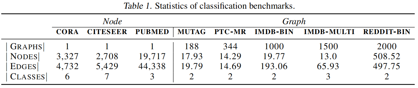
Benchmarks as above.

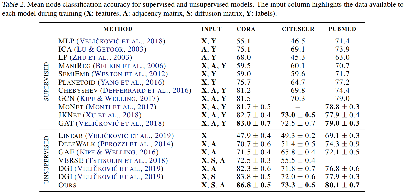
Node classification.

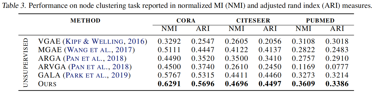
Clustering.

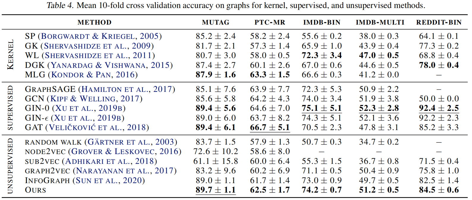
Graph classification.

Five contrastive modes:

local-global: contrast node encodings from one view with graph encodings from the other;
global-global: contrast graph encodings across views;
multi-scale: contrast graph encodings from one view with intermediate encodings from the other; intermediate encodings use DiffPool;
hybrid: combine local-global and global-global;
ensemble modes: for all views, contrast node and graph encodings from the same view.

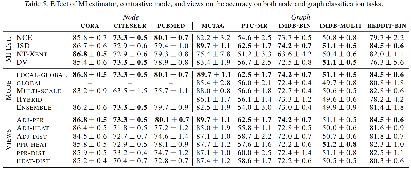
Results in Table 5 show that contrasting node and graph encodings consistently performs best across benchmarks. This highlights an important difference between graph and visual representation learning:

1) In visual representation learning, contrasting global views works best; on graphs, contrasting node and graph encodings works better for both node and graph classification.

2) Multi-scale contrast helps visual representation learning but hurts graph representation learning.

Yang Tan (谭扬)